Computing curvature is a common problem that has applications in a variety of areas from computational physics to computer graphics to machine learning. In this post I’m going to cover the main ideas behind my recent paper in which I propose a novel algorithm (VWME) for robustly computing curvature.
Going forward we’ll be focusing on a particular variant of the curvature problem in which the only information we’re provided is point cloud data which may be of arbitrary dimension. This is different from what is typical in computer graphics where one is usually constrained to three dimensions and has additional mesh information connecting the point cloud points to form a surface.
The idea is essentially to solve the problem in three parts; construct an surface from the point cloud data, determine the surface normals, then use this information to determine the curvature of the surface at any given point. Many readers may realize that this is essentially a problem of Manifold Learning.
Surface Estimation
When just provided with point cloud data there are a few different methods for estimating a surface based on the observed points. The methods we considered in the VWME algorithm include the $\varepsilon-$ball method, KNN method, and RBF kernel method. We’ll explain what these methods are but what’s really important is that these are all just methods of connecting a point to other points nearby. These connected points form a graph which is our surface!
$\varepsilon-$ball Method
This method entails simply constructing an $\varepsilon-$ball around each point and connecting that point to all the other points within that ball. This method is quite simply; however, it has a lot issues with leaving disconnected points when the point cloud isn’t densely sampled. Essentially, for a given point $x_i \in x$ it’s neighbors are defined as $N(x_i) = \{x : |x-x_i| < \varepsilon \}$ given some $\varepsilon$ we’ve chosen.
KNN Method
The KNN Method uses the K-Nearest Neighbors algorithm to find the $K$ nearest points to a given point and connects them. It’s worth noting that this method is not necessary reflexive so we will likely end up with points with more than $K$ edges. This is also among the most popular algorithms for manifold estimation from point cloud data because it solves the sparse sampling problem associated with the $\varepsilon-$ball method; however, it doesn’t benefit from as many theoretical guarantees.
RBF Kernel Method
The RBF Kernel Method works by applying a Gaussian Radial Basis Function Kernel from every point in the point cloud to every other point in the cloud. Essentially, this creates a densely connected graph with edge weights given by the RBF kernel so farther points have “weaker” edges. In many of my personal experiments this method is the most robust to noise but, since the graph is fully connected, it is computationally infeasible for even moderately sized point clouds. So we form a fully connected graph with edge weights $W(x_i,x_j) = \exp \bigg(-\frac{||x_i - x_j||^2}{2\sigma^2}\bigg)$ where $\sigma$ is a parameter we have to choose and tune.
Curvature Estimation
Now that we have turned the point cloud into some sort of surface we can begin to approximate the curvature of the surface. In the case of the VWME algorithm proposed in my paper and in similar algorithms, this is done by first determining the normal vectors to the surface and then observing how they change. This change in normal vectors gives us information that allows us to estimate the curvature of the surface.
Weingarten Map Estimator
The algorithm that VWME is an improvement on is the Weingarten Map Estimator (WME). The Weingarten Map or Shape Operator is a linear operator on a manifold that encapsulates the change in the normal vector of said manifold. This is useful because determining the Weingarten Map then allows us to derive and compute various types of curvature from it. The WME algorithm works by, given a normal vector at each point, linearly approximating the Weingarten Map as some function of the change in the local normal vectors. Solving this problem ends up being equivalent to solving a linear least squares problem.
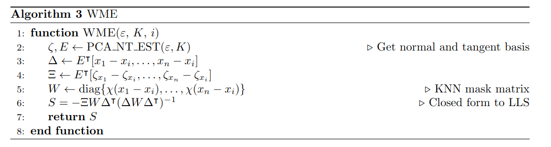
Above we see the exact algorithm used for this estimation which we’ll walk through. The first step involves estimating the normal vectors of the surface using a form of PCA which results in $\zeta$ (our normal vectors) and $E$ (our tangent space). We then do a change of basis for the bracketed terms to form the matrices $\Delta$ and $\Xi$. All that’s left is to apply the matrix $W$ which filters the data to only allow nearby points (in this example we use K nearest neighbors for this) then use the closed form of linear least squares to solve for our Weingarten map $S$.
Voronoi Weingarten Map Estimator
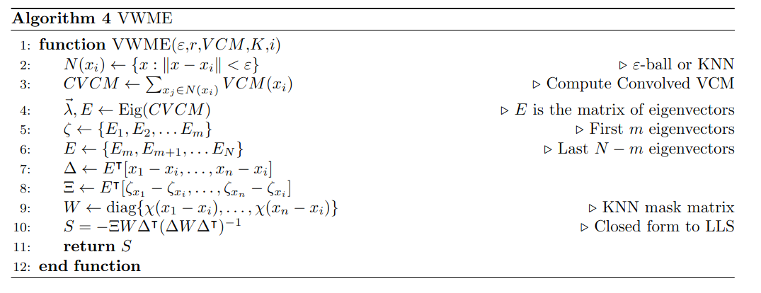
Here we have our proposed VWME algorithm which serves to improve upon the WME algorithm. You’ll probably notice that this algorithm is quite similar with the primary difference being in how the normal vectors are computed. In the WME algorithm it is assumed that the point cloud data is noiseless and we are able to exactly reconstruct the normal vectors using local PCA. Unfortunately, this is often not the case in real world data which is why we introduced a robustness improvement to this algorithm which leverages a robust metric called the Voronoi Covariance Measure which, for the purpose of this article, can just be thought of as a metric that can lead to more robust estimation of normal vectors. As it turns out, the eigenvectors of the VCM are good estimates of the normal and tangent space of our manifold. Using this VCM method we augmented the traditional WME algorithm to more accurately compute curvature of various surfaces given noisy data.
Results
The first results we’ll see are some visual examples of curvature estimations using the traditional WME algorithm below
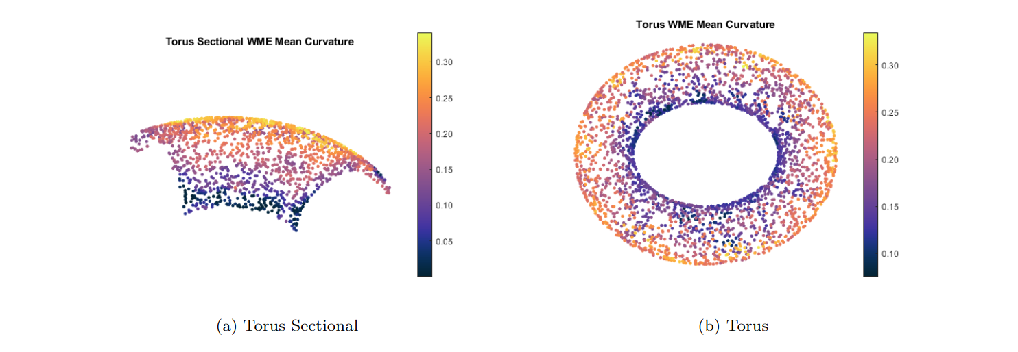
So here we have a fairly densely sampled torus (and torus sectional) where we can see how the algorithm does at estimating the mean curvature across the entire surface. Overall the standard WME algorithm does a good job at estimating this curvature; however, there are several instances where points are given the wrong curvature despite surrounding points being correctly estimated.
Since the curvature of the torus is known analytically, after introducing our VWME algorithm we can compare how well the algorithms do at estimating it.
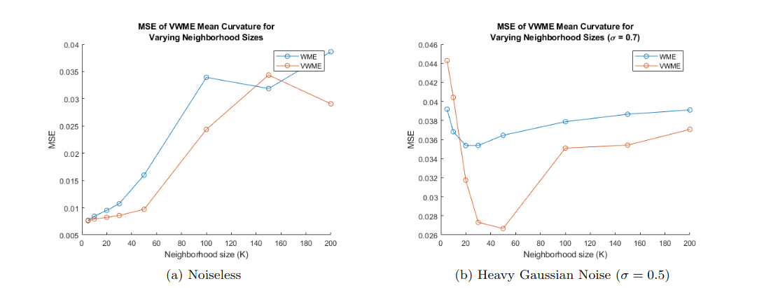 After running these algorithsm head to head we see that VWME comes out on top in both the noisy and noiseless cases! This is great news; however, a bit surprising for the noiseless case but further investigation explains this as well. Even in the case of no noise the VCM estimator is slightly better than local PCA for determining normal vectors because local PCA has a greater propensity towards “flipping” the normals. Essentially, PCA will correctly determine the angle of the normal vectors but 180 degrees off so the vector is facing backwards. This error propagates through the algorithm and causes and increase in WME curvature error.
Anyways, that’s the basics behind curvature estimation for point cloud data. If you’re interested in reading further into how exactly this works (and why) feel free to read my paper which covers everything more thoroughly (albeit with a bit of differential geometry)!