We begin by continuing from where we left off in the previous post. We’ll be performing some further analysis on the Valorant competitive data we processed and revisit our goal of determining the best competitive team composition.
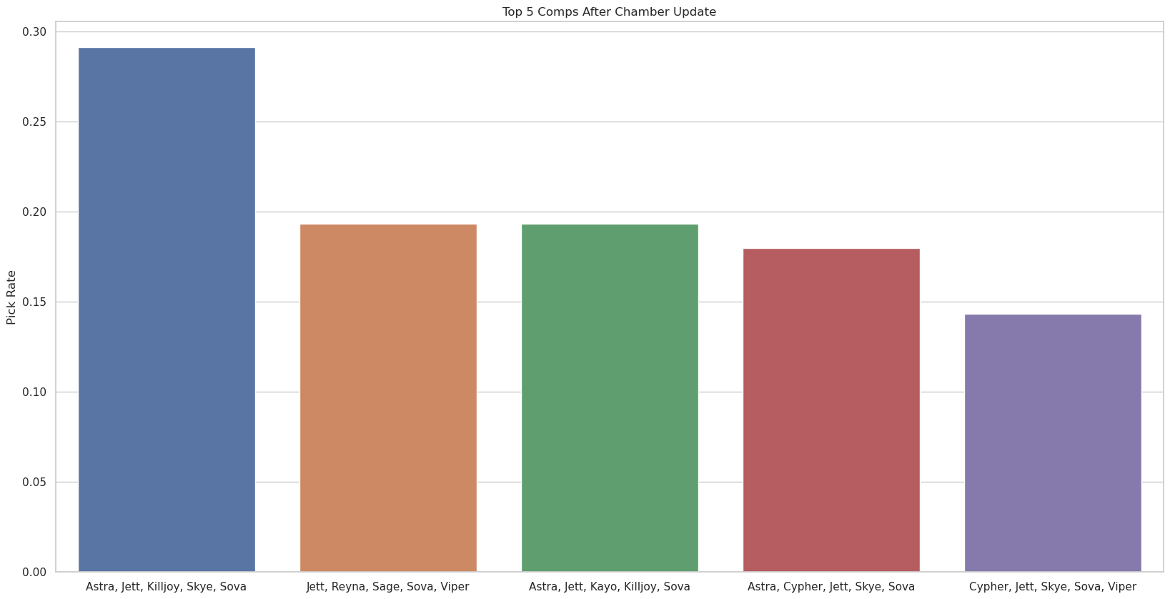
In the previous post we ended after we were able to determine the most popular agents by update. Now we consider one particular update (the Chamber update here) and plot the most popular agent compositions used in the pro matches during this update period.
def keys_to_str(x):
    result = ""
    for agent in x:
        result += str(agent)[0].upper() + str(agent)[1:] + ", "
    return result[:-2]

# Top three team comps for chamber update
plt.cla()
plt.clf()
sns.set_theme(style="whitegrid")
n = 5 # number of comps to plot
ms = sorted(team_pick_by_milestone.keys())[0]
ordered_picks = sorted(team_pick_by_milestone[ms].items(), key=lambda x : -x[1])
top_three = ordered_picks[:n]
packed_teams = list(zip(*top_three))
comp, counts = packed_teams[0], packed_teams[1]
total_games = sum(counts)
comp_name = [keys_to_str(x) for x in comp]
plt.figure(figsize=(4*n,10))
plt.title(f"Top {n} Comps After Chamber Update")
plt.ylabel('Pick Rate')
ax = sns.barplot(x=np.array(comp_name), y=np.array(counts) / total_games)
plt.show()
Finally, we can compute the winrate for each of the team compositions
def drop_dupes(seq):
    seen = set()
    seen_add = seen.add
    return [x for x in seq if not (x in seen or seen_add(x))]

# Get winrate by team comp
# Convert Abbreviation to Team ID
game_ids_idx = tqdm(game_ids)
team_winrate_by_milestone = dict()
team_gamecount_by_milestone = dict()
team_wins_by_milestone = dict()
for cluster in adjusted_clusters:
    team_winrate_by_milestone[cluster] = defaultdict(lambda : 0)
    team_gamecount_by_milestone[cluster] = defaultdict(lambda : 0)
    team_wins_by_milestone[cluster] = defaultdict(lambda : 0)
for game_id in game_ids_idx:
    df_gs =  dataframes["game_scoreboard"]
    cur_game_df = df_gs.loc[df_gs["GameID"] == game_id]
    teams = drop_dupes(list(cur_game_df["TeamAbbreviation"]))
    teams = [x for x in teams if len(x) > 0]
    if len(teams) != 2: # we are missing data so we must skip the datapoint
        continue
    df_g = dataframes["games"]
    cur_game_g_df = df_g.loc[df_g["GameID"] == game_id]
    team_count = 0
    for t in teams:
        team_count += 1

        t_comp = cur_game_df.loc[cur_game_df["TeamAbbreviation"] == t]["Agent"]
        t_comp_list = t_comp.tolist()
        if len(t_comp_list) != 5 or '' in t_comp_list:
            continue
        # Get team ID
        df_g = dataframes["games"]
        team_id = cur_game_g_df[f"Team{team_count}ID"]
        won = False
        won = True if cur_game_g_df["Team1_TotalRounds"].tolist()[0] > cur_game_g_df["Team2_TotalRounds"].tolist()[0] else False
        if team_count != 1:
            won = not won
        date_days = (last_match_date - game_id_to_date[game_id]).days
        try:
            milestone = date_to_milestone(date_days)
        except:
            print("Comp:", t_comp)
            print("Date_days:", date_days)
        for agent in t_comp_list:
            agent_pick_by_milestone[milestone][agent] += 1
        team = sorted(t_comp.tolist())
        team_pick_by_milestone[milestone][tuple(team)] += 1
        team_gamecount_by_milestone[milestone][tuple(team)] += 1
        if won:
            team_winrate_by_milestone[milestone][tuple(team)] += 1
            team_wins_by_milestone[milestone][tuple(team)] += 1
# Normalize
for ms in team_winrate_by_milestone.keys():
    for team in team_winrate_by_milestone[ms].keys():
        team_winrate_by_milestone[ms][team] /= team_gamecount_by_milestone[ms][team]
So now we’ve taken the data and processed it to compute the winrate for each team composition, for each update, based on what we’ve been told by our dataset. However, whether one team beats another is itself a random process for which we have a limited set of data so there is noise inherent to our data. In order to account for this we can compute confidence intervals for our winrate calculations.
# Compute 95% confidence intervals
import scipy.stats as st

team_winrate_ci_by_milestone = dict()
for cluster in adjusted_clusters:
    team_winrate_ci_by_milestone[cluster] = defaultdict(lambda : 0)
for ms in team_winrate_by_milestone.keys():
    for team in team_winrate_by_milestone[ms].keys():
        temp_data = np.zeros(team_gamecount_by_milestone[ms][team])
        wins = np.round(team_winrate_by_milestone[ms][team] * team_gamecount_by_milestone[ms][team]).astype(int)
        temp_data[:wins] = np.ones(wins)
        if team_gamecount_by_milestone[ms][team] > 30:
            team_winrate_ci_by_milestone[ms][team] = st.norm.interval(alpha=0.95, loc=team_winrate_by_milestone[ms][team], scale=st.sem(temp_data))
        else:
            team_winrate_ci_by_milestone[ms][team] = st.t.interval(alpha=0.95, df=len(temp_data)-1, loc=team_winrate_by_milestone[ms][team], scale=st.sem(temp_data))
Then we can plot the results with the confidence intervals demonstrating the uncertainty in our data. You’ll notice that we choose to use a 95% confidence interval and that when computing the confidence intervals for the data we only use a noraml distribution for the interval once we’ve exceeded 30 samples. This is because the central limit theorem does not converge fast enough for a normal distribution to be a good representation of the sparsely sampled data below this so we use the t-distribution in this case due to its fatter tails.
# Get comps with the highest win-rate
plt.cla()
plt.clf()
n = 6 # number of comps to plot
required_plays = 50 # number of required uses
ms = sorted(team_winrate_by_milestone.keys())[0]
ordered_picks = sorted(filter(lambda x : team_gamecount_by_milestone[ms][x[0]] > required_plays, team_winrate_by_milestone[ms].items()), key=lambda x : -x[1])

top_n = ordered_picks[:n]
packed_teams = list(zip(*top_n))
err_interval = list()
for i in range(len(packed_teams[0])):
    err_interval.append(list(team_winrate_ci_by_milestone[ms][packed_teams[0][i]]) )
comp, counts = packed_teams[0], packed_teams[1]
total_games = sum(counts)
comp_name = [keys_to_str(x) for x in comp]
plt.figure(figsize=(4*n,10))
plt.title(f"Top {n} Comps by Winrate After Chamber Update")
plt.ylabel('Winrate')
sns.set_theme(style="whitegrid")
err_interval = np.array(err_interval,dtype=np.float32)
ci_interval = (err_interval[:,1] - err_interval[:,0]) / 2
ax = sns.barplot(x=np.array(comp_name), y=np.array(counts), capsize=0.1, yerr=ci_interval)
plt.show()
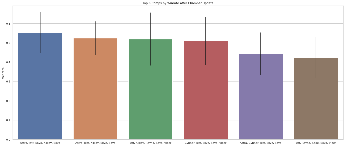
So now we’ve produced a nice plot of the “best” team compositions immediately following the Chamber update; however, there’s a few caveats worth noting. In particular, we’ve chosen to plot 6 teams and you may have noticed that these teams don’t even have the highest win rates! So why have we chosen them? Well, we have to filter the data because there are several team compositions with 100% win rates simply due to the fact that they’ve only been used once or twice.
After thinking about this a bit we realize that we’re not really interested in finding the team composition with the highest win rate; but rather, we want the team compositions that are the best (i.e. the most likely to win). Looking at our confidence intervals for these seldom used, extreme win rate teams, shows us that there’s no confidence at all in the computed win rate so we have to throw this data out.
As a result, we’ve only considered fairly popular team compositions that have been played at least 50 times and get the result we see above. We’ll note that the lower bound on the confidence intervals for these win rates are almost entirely monotonically decreasing which is exactly what we like to see!
Now that we’ve determined the “best” team compositions for this update we might also want to know whether the more popular team compositions are actually better. Essentially, are the pros making the right decisions in choosing their team compositions? (there are several complications that make this incredibily difficult to reliably answer which we’ll discuss but we can at least try)
# Does team comp popularity correlate with win rate?

import scipy.stats as st

plt.cla()
plt.clf()
ms = sorted(team_winrate_by_milestone.keys())[0] # choose a milestone
winrate_list = list()
popularity = list()
for team in team_winrate_by_milestone[ms]:
    winrate_list.append(team_winrate_by_milestone[ms][team])
    popularity.append(team_gamecount_by_milestone[ms][team])

winrate_arr = np.array(winrate_list)
popularity_arr = np.array(popularity)
scatter_df = pd.DataFrame({"WinRate":winrate_arr, "Popularity":popularity_arr})
r, p = st.pearsonr(popularity_arr, winrate_arr)
sns.lmplot(x="WinRate", y="Popularity", data=scatter_df)
plt.title("Are Popular Team Comps Better?")

plt.show()
print("Correlation (Pearson-R):", r)
print("P-value:", p)
Correlation (Pearson-R): -0.25791594975765486
P-value: 0.0038274956553406977
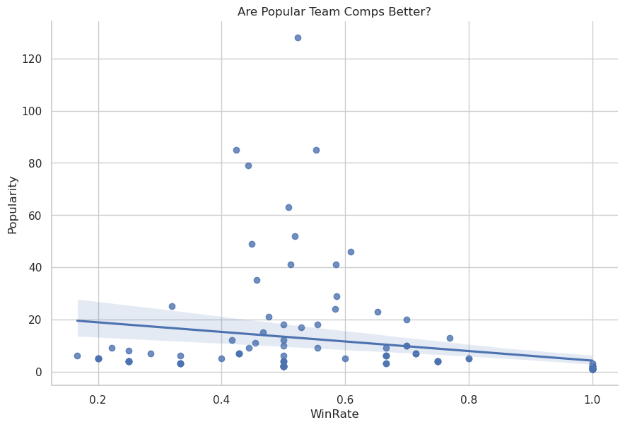
So we see when considering all the possible team comps that there is actually a negative correlation between popularity and win rate! This seems a bit strange; however, we have to realize that a lot of the data is just complete noise as we found out when determining the confidence intervals for low popularity data points.
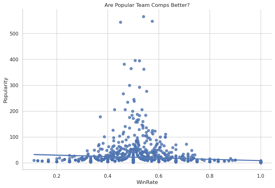
This is problematic since low popularity team compositions have inherently less certainty so we can’t accurately compute their correlation with win rate. The first thing we can try is to redo the calculation using all the data across every update the game has resulting in the following
Correlation (Pearson-R): -0.14297965158342224
P-value: 2.0711792457434896e-08
After thinking about this a bit more we realize that since many of the data points have a lot of uncertainty we should just treat them as distributions rather simply taking the mean value we’re using as our sample point. We can accomplish this by performing a Monte Carlo simulation of the data points.
# Correlation Monte Carlo Simulation
# -----------------------------------
# Simulates each winrate datapoint
# with an estimator matching mean &
# variance based on count
#
# For n > 30 central limit theorem
# should give good approx w/ normal
# distribution
#
# For n < 30 we can use binomial
# distribution as these are a series
# of bernoulli RV's
# ----------------------------------
nan_bound = 0
binom_bound = 30
sim_count = 10000
ms_list = sorted(team_winrate_by_milestone.keys())
spearman_r = np.zeros(sim_count)
spearman_p = np.zeros(sim_count)
pearson_r = np.zeros(sim_count)
pearson_p = np.zeros(sim_count)
sim_indices = tqdm(range(sim_count))
for j in sim_indices:
    winrate_sim = np.zeros(len(winrate_arr))
    i = 0
    for ms in ms_list:
        for team in team_winrate_by_milestone[ms]:
            if popularity_arr[i] > binom_bound:
                mean = winrate_arr[i]
                run = np.zeros(team_gamecount_by_milestone[ms][team])
                count = popularity_arr[i]
                run[:count] = np.ones(count)
                var = np.var(run)
                winrate_sim[i] = np.random.normal(loc=mean, scale=np.sqrt(var)/count)
            elif popularity_arr[i] > nan_bound:
                count = popularity_arr[i]
                mean = winrate_arr[i]
                winrate_sim[i] = np.random.binomial(n=count,p=mean) / count
            else:
                winrate_sim[i] = np.NAN
            i += 1
    winrate_sim_clean, pop_clean = zip(*filter(lambda x : not np.isnan(x[0]), zip(winrate_sim, popularity_arr)))
    scatter_df = pd.DataFrame({"WinRate":winrate_sim_clean, "Popularity":pop_clean})
    r, p = st.pearsonr(pop_clean, winrate_sim_clean)
    sr, sp = st.spearmanr(pop_clean, winrate_sim_clean)
    pearson_r[j] = r
    pearson_p[j] = p
    spearman_r[j] = sr
    spearman_p[j] = sp
Now that we’ve done the Monte Carlo simulation of 10,000 samples we can plot the distributions we have for the Correlation Coefficient (Pearson-R) and the P-Value of this computation.
plt.cla()
plt.clf()

# ------- Pearson-R --------

plt.figure(figsize=(10,10))
plt.title(f"Pearson-R Distribution")
plt.ylabel('Probability')
plt.xlabel('Pearson-R')
sns.set_theme(style="whitegrid")

ax = sns.histplot(x=np.array(pearson_r), bins=10, stat='probability')
plt.show()

# ------- P-Value ----------

plt.figure(figsize=(10,10))
plt.title(f"Pearson P-value Distribution")
plt.ylabel('Probability')
plt.xlabel('P-value')
sns.set_theme(style="whitegrid")

ax = sns.histplot(x=np.array(pearson_p), bins=10, stat='probability')
plt.show()

print(f"Mean Pearson-R: {np.mean(pearson_r)}")
print(f"Mean P-value: {np.mean(pearson_p)}")
Mean Pearson-R: -0.11536534278545539
Mean P-value: 1.031394866067974e-05
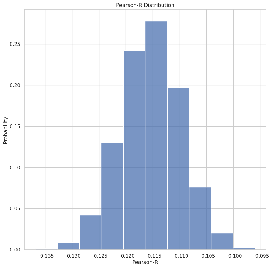
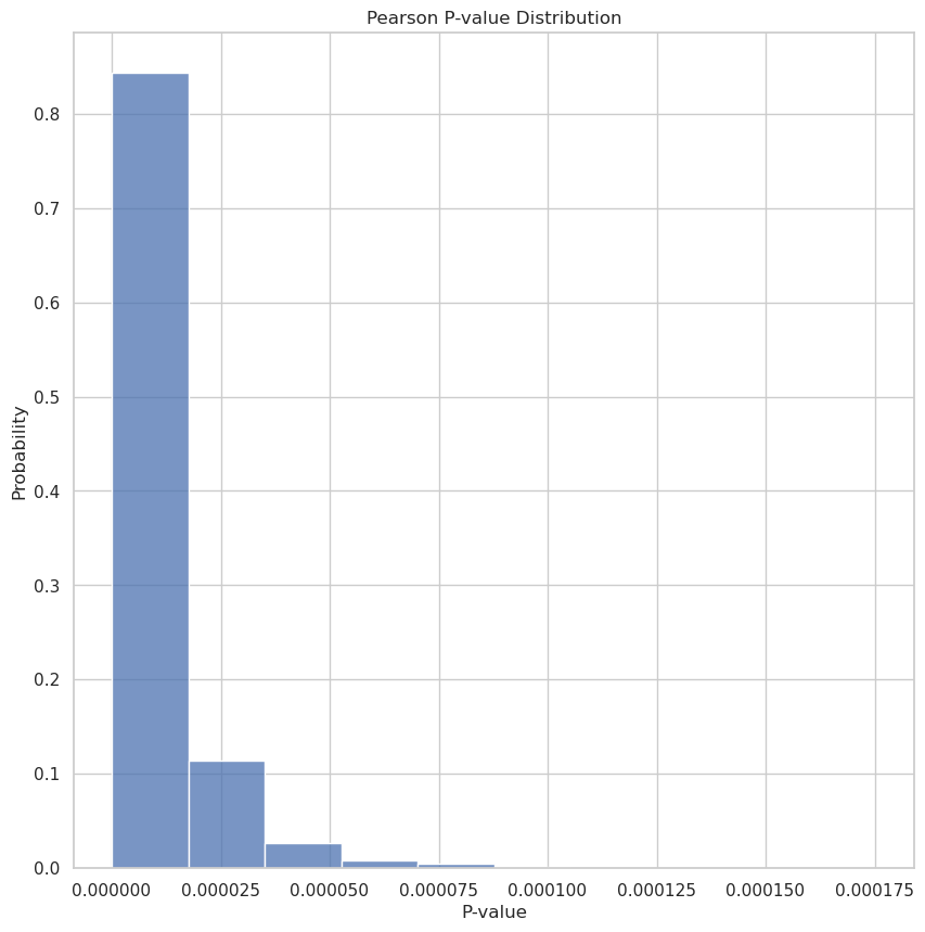
Looking at these graphs we do, in fact, see there is a negative correlation between team popularity and win rate! Looking at the P-value distribution we also note that the P-value is certainly less than 0.05 with high probability.
It’s worth noting that when we remove the team comps only played once this correlation disspears and becomes functionally zero. This indicates that the best strategy for professional Valorant is to play a team comp that has never been played before; however, once it’s been seen it seems to lose any competitive edge.