In this post we’ll be going through an SQL database of professional valorant stats, process that data, and use the results to try and determine what the best team comps are. Before we begin, if you want to follow along, the dataset can be downloaded here.
Now that we have the sql database we can begin by importing it into python.
import sqlite3
import pandas as pd
from collections import defaultdict
from tqdm.notebook import tqdm
import sklearn

con = sqlite3.connect('valorant.sqlite')
cursor = con.cursor()
cursor.execute("SELECT name FROM sqlite_master WHERE type='table';")
tables = cursor.fetchall()
table_names = [table[0] for table in tables]
print(f"TABLES:\n {table_names}")
 TABLES:
 ['Matches', 'Games', 'Game_Rounds', 'Game_Scoreboard']
We can then further examine the structure of the SQL database to see exactly what we’re working with
dataframes = {}
for table in table_names:
    dataframes[table.lower()] = pd.read_sql_query(f"SELECT * FROM {table}", con)

for df_name, df in dataframes.items():
    print(f"{df_name}:\n {list(df.columns)}\n")
matches:
 ['MatchID', 'Date', 'Patch', 'EventID', 'EventName', 'EventStage', 'Team1ID', 'Team2ID', 'Team1', 'Team2', 'Team1_MapScore', 'Team2_MapScore']

games:
 ['GameID', 'MatchID', 'Map', 'Team1ID', 'Team2ID', 'Team1', 'Team2', 'Winner', 'Team1_TotalRounds', 'Team2_TotalRounds', 'Team1_SideFirstHalf', 'Team2_SideFirstHalf', 'Team1_RoundsFirstHalf', 'Team1_RoundsSecondtHalf', 'Team1_RoundsOT', 'Team2_RoundsFirstHalf', 'Team2_RoundsSecondtHalf', 'Team2_RoundsOT', 'Team1_PistolWon', 'Team1_Eco', 'Team1_EcoWon', 'Team1_SemiEco', 'Team1_SemiEcoWon', 'Team1_SemiBuy', 'Team1_SemiBuyWon', 'Team1_FullBuy', 'Team1_FullBuyWon', 'Team2_PistolWon', 'Team2_Eco', 'Team2_EcoWon', 'Team2_SemiEco', 'Team2_SemiEcoWon', 'Team2_SemiBuy', 'Team2_SemiBuyWon', 'Team2_FullBuy', 'Team2_FullBuyWon']

game_rounds:
 ['GameID', 'Team1ID', 'Team2ID', 'RoundHistory']

game_scoreboard:
 ['GameID', 'PlayerID', 'PlayerName', 'TeamAbbreviation', 'Agent', 'ACS', 'Kills', 'Deaths', 'Assists', 'PlusMinus', 'KAST_Percent', 'ADR', 'HS_Percent', 'FirstKills', 'FirstDeaths', 'FKFD_PlusMinus', 'Num_2Ks', 'Num_3Ks', 'Num_4Ks', 'Num_5Ks', 'OnevOne', 'OnevTwo', 'OnevThree', 'OnevFour', 'OnevFive', 'Econ', 'Plants', 'Defuses']
Now we can move onto the real question that we’re all wondering - is there a best Valorant team comp? And if so what is it? In order to answer these questions we need to do a little bit of data processing and cleaning so we have the information we need to proceed. This can take some time so we wrap it in a tqdm function to see the progress.
comp_dict = dict() # maps sorted agent comp to win count
game_ids = dataframes["game_scoreboard"]["GameID"].drop_duplicates()
df_gs = dataframes["game_scoreboard"]
comps = defaultdict(lambda : 0) # map from teams to number of games
game_ids_idx = tqdm(game_ids) # tqdm for progress
for game_id in game_ids_idx:
    cur_game_df = df_gs.loc[df_gs["GameID"] == game_id]
    teams = list(cur_game_df["TeamAbbreviation"].drop_duplicates())
    teams = [x for x in teams if len(x) > 0]
    if len(teams) != 2: # missing data so skip
        continue
    for t in teams:
        t_comp = cur_game_df.loc[cur_game_df["TeamAbbreviation"] == t]["Agent"]
        t_comp_list = t_comp.tolist()
        if len(t_comp_list) != 5 or '' in t_comp_list:
            continue
        team = sorted(t_comp.tolist())
        comps[tuple(team)] += 1
It will also be useful to us to determine how often each of the agents are used so we’ll go ahead and compute that
agent_count = defaultdict(lambda : 0)
for key in comps.keys():
    for agent in key:
        agent_count[agent] += 1
However, there’s a slight problem with this approach; not all the playable agents in Valorant have existed from the beginning of the game. In fact, a large number of them were added later on so we have to normalize by the time each agent has existed. To get this timeframe we simply iterate through all the games and compute the first and last match dates for each of the agents.
from datetime import datetime, date
agent_add_date = defaultdict(lambda : datetime.max)
game_id_to_date = dict()
game_ids_idx = tqdm(sorted(game_ids) )
first_match_date = None
last_match_date = None
for game_id in game_ids_idx:
    df_gs = dataframes["game_scoreboard"]
    cur_game_scoreboard_df = df_gs.loc[df_gs["GameID"] == game_id]
    agents = cur_game_scoreboard_df["Agent"].unique()

    df_games = dataframes["games"]
    cur_game_df = df_games.loc[df_games["GameID"] == game_id]
    match_id = cur_game_df["MatchID"].unique()[0]
    match_id_df = dataframes["matches"].loc[dataframes["matches"]["MatchID"] == match_id]
    date_data = match_id_df["Date"].unique()[0]
    datetime_data = datetime.strptime(date_data, "%Y-%m-%d %H:%M:%S")
    game_id_to_date[game_id] = datetime_data
    if first_match_date is None or datetime_data < first_match_date:
        first_match_date = datetime_data
    if last_match_date is None or datetime_data > last_match_date:
        last_match_date = datetime_data
    for agent in agents:
        # found first instance of agent
        # check len() for removing bad data
        if len(agent) > 1 and datetime_data <= agent_add_date[agent]:
            agent_add_date[agent] = datetime_data
Then we can get the total time each of the agents has existed
agent_times = dict()
for agent, add_date in agent_add_date.items():
    agent_times[agent] = (last_match_date - add_date).days
print("Original Agent Times:", agent_times)
Original Agent Times:
{'reyna': 583, 'cypher': 597, 'omen': 594, 'raze': 597, 'sova': 597, 'phoenix': 597, 'jett': 597, 'killjoy': 513, 'breach': 597, 'sage': 597, 'viper': 583, 'brimstone': 597, 'skye': 428, 'yoru': 345, 'astra': 294, 'kayo': 184, 'chamber': 42}
Another problem is that since agents are only released with major updates it’s unlikely that we would get a large number of similar but still different values for agent existence times. This is due to noise in our dataset and we can resolve it by clustering.
Essentially, we cluster agents based on when we first see them. If their times are sufficiently close (e.g. in the same cluster) then we can tell they were actually available at the same time so we set their “release” time to the earliest value in the cluster. In order to actually perform the clustering we can just go with the standard K-means data mining approach with K chosen based on our knowledge of the game and how frequently new agents are released.
import numpy as np
from sklearn.cluster import KMeans
milestones = np.array([int(x) for x in agent_times.values()])
clusters = 7
kmeans = KMeans(n_clusters=clusters).fit(milestones.reshape(-1,1))
print("Clusters:\n",kmeans.cluster_centers_)
print()
cluster_map = defaultdict(lambda : [])
for agent, time in agent_times.items():
    cluster_map[int(kmeans.predict(np.array(time).reshape(-1,1) ))].append(agent)
adjusted_agent_times = dict()
for key in cluster_map.keys():
    for agent in cluster_map[key]:
        adjusted_agent_times[agent] = max([agent_times[a] for a in cluster_map[key]])
print("Adjusted Agent Times:", adjusted_agent_times)
adjusted_clusters = sorted(list(set(adjusted_agent_times.values())))
print("Adjusted Clusters:", adjusted_clusters)
Clusters:
 [[594.18181818]
 [294.        ]
 [ 42.        ]
 [428.        ]
 [184.        ]
 [513.        ]
 [345.        ]]

Adjusted Agent Times: {'reyna': 597, 'cypher': 597, 'omen': 597, 'raze': 597, 'sova': 597, 'phoenix': 597, 'jett': 597, 'breach': 597, 'sage': 597, 'viper': 597, 'brimstone': 597, 'killjoy': 513, 'skye': 428, 'yoru': 345, 'astra': 294, 'kayo': 184, 'chamber': 42}
Adjusted Clusters: [42, 184, 294, 345, 428, 513, 597]
So now that we have these updates or “milestones” in which new agents are introduced we can determine agent and total comp pick rate across each of these updates.
def date_to_milestone(date_days):
    milestone = adjusted_clusters[0]
    for i in range(len(adjusted_clusters)):
        if i == 0 and date_days <= adjusted_clusters[0]:
            return adjusted_clusters[0]
        if date_days > adjusted_clusters[i-1] and date_days <= adjusted_clusters[i]:
            return adjusted_clusters[i]
    raise Exception(f"Error: {date_days}")
game_ids_idx = tqdm(game_ids)
agent_pick_by_milestone = dict()
team_pick_by_milestone = dict()
for cluster in adjusted_clusters:
    agent_pick_by_milestone[cluster] = defaultdict(lambda : 0)
    team_pick_by_milestone[cluster] = defaultdict(lambda : 0)
for game_id in game_ids_idx:
    df_gs =  dataframes["game_scoreboard"]
    cur_game_df = df_gs.loc[df_gs["GameID"] == game_id]
    teams = list(cur_game_df["TeamAbbreviation"].drop_duplicates())
    #print(teams)
    teams = [x for x in teams if len(x) > 0]
    if len(teams) != 2: # missing data so skip
        continue
    for t in teams:
        t_comp = cur_game_df.loc[cur_game_df["TeamAbbreviation"] == t]["Agent"]
        t_comp_list = t_comp.tolist()
        if len(t_comp_list) != 5 or '' in t_comp_list:
            continue
        date_days = (last_match_date - game_id_to_date[game_id]).days
        try:
            milestone = date_to_milestone(date_days)
        except:
            print("Comp:", t_comp)
            print("Date_days:", date_days)
        for agent in t_comp_list:
            agent_pick_by_milestone[milestone][agent] += 1
        team = sorted(t_comp.tolist())
        team_pick_by_milestone[milestone][tuple(team)] += 1
Now we can finally create our first graphs of agent popularity by update and we can even color the graph by the agent’s colors with the following code
agent_to_color = {
    'jett' : 'cornflowerblue',
    'chamber' : 'goldenrod',
    'sova' : 'lightsteelblue',
    'viper' : 'limegreen',
    'skye' : 'springgreen',
    'astra' : 'rebeccapurple',
    'raze' : 'darkorange',
    'sage' : 'aquamarine',
    'kayo' : 'dodgerblue',
    'killjoy' : 'yellow',
    'reyna' : 'orchid',
    'cypher' : 'dimgrey',
    'breach' : 'coral',
    'omen' : 'darkslateblue',
    'brimstone' : 'chocolate',
    'phoenix' : 'orangered',
    'yoru' : 'royalblue'
}

import matplotlib.pyplot as plt
import seaborn as sns
sns.set_theme(style="darkgrid")
for milestone, picks in agent_pick_by_milestone.items():
    items = sorted(picks.items(), key=lambda x : -x[1])
    packed = list(zip(*items))
    agents, counts = packed[0], packed[1]
    colors = [agent_to_color[a] for a in agents]
    plt.figure(figsize=(18,9))
    plt.title(f'Update {milestone}')
    plt.ylabel('Count')
    ax = sns.barplot(x=np.array([str(a[0]).upper() + a[1:] for a in agents]), y=np.array(counts), palette = colors)
    plt.show()
Now we can look at a couple of the graphs we get out and see if the results so far make sense,
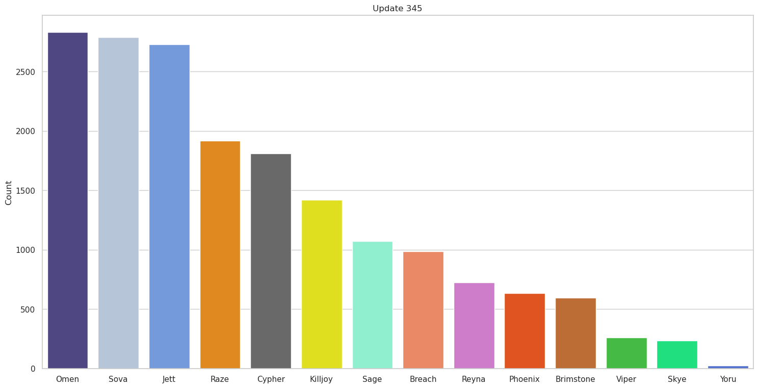
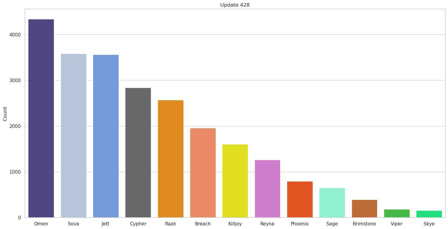
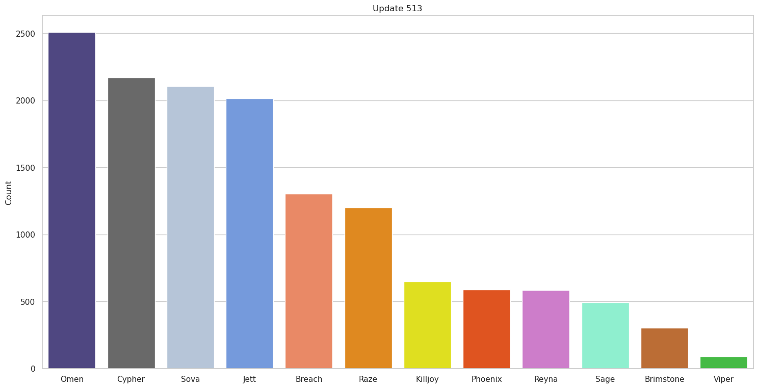
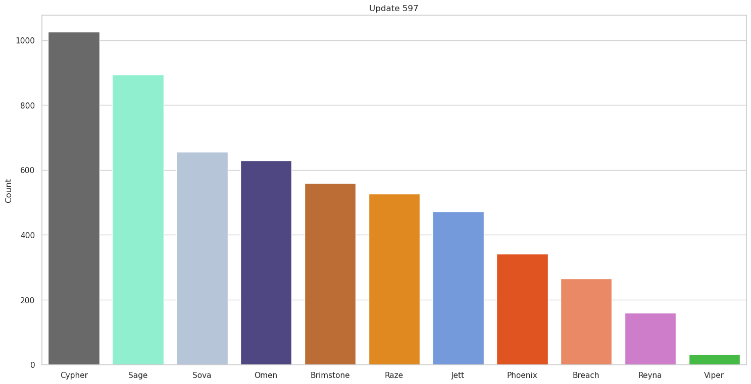
So far so good, this seems to generally match what we would expect based on what we know of competitive team comps at the time. It’s also interesting to see how some agents change spots across updates; for instance, the decline in Jett use as she was nerfed makes perfect sense. We also see some teams initially tested out Yoru; however, it was quickly discovered he simply wasn’t good in professional matches and stopped being used at all.
That’s all there is for part 1, in part 2 we’ll really dive into some analysis and actually see if we can figure what the best team comps are! You read part 2 here.